How Regressions Work: A Simple Guide to Y, X, Alpha and Factor Models
Regression analysis is used throughout investment research. It appears in academic papers, fund analysis, performance attribution and discussions about whether an active manager has produced genuine alpha. It is also central to factor models such as the Capital Asset Pricing Model and the Fama–French three-factor and five-factor models.
Despite this, regressions can initially look more complicated than they really are. The equations contain unfamiliar letters, Greek symbols and statistical terms such as dependent variables, explanatory variables, coefficients, intercepts, residuals, standard errors, t-statistics and R².
At the most basic level, though, a regression is simply a way of measuring how changes in one thing are related to changes in one or more other things.
In finance, we might ask:
‘How much of this fund’s return can be explained by movements in the stock market?’
A Fama–French regression asks a broader question:
‘How much of this fund’s return can be explained by its exposure to the market, smaller companies, value companies and other systematic factors?’
The regression examines a series of historical observations and estimates the combination of relationships that comes closest to explaining the results.
This article begins with the simplest possible regression, containing one variable that we want to explain and one variable that we use to explain it. It then builds towards a Fama–French factor regression and explains how to interpret alpha, factor loadings, residuals, R², standard errors and t-statistics.
The Basic Regression Equation
The simplest regression equation is:
Y = alpha + beta X + error
Each part has a specific meaning.
Y = The variable being explained
X = The variable used to help explain Y
alpha = The intercept
beta = The estimated relationship between X and Y
error = The part of Y that the regression does not explain
The letters themselves are not particularly important. What matters is understanding the role each part plays.
Y: The Dependent Variable
Y is the thing the regression is trying to explain.
It is called the dependent variable because its estimated value depends on the values of the other variables included in the model.
In an investment regression, Y might be:
a fund’s monthly return;
a stock’s monthly return;
a portfolio’s monthly return;
the return above a benchmark;
or the return above the risk-free rate.
In a standard factor regression, Y is normally the investment’s excess return.
Investment excess return = Investment return - Risk-free return
Suppose a fund returns 1.20% during a month and the risk-free return is 0.30%. Fund excess return = 1.20% - 0.30%. Fund excess return = 0.90%. The Y-value for that month is therefore 0.90%.
The risk-free return is deducted because factor models generally seek to explain the return earned above the return available on a relatively risk-free asset. The model is not trying to explain the entire return. It is trying to explain the additional return associated with taking investment risk.
The subscript t is often added to show that a value relates to a particular time period.
Yₜ = the value of Y in period t
If monthly data are being used, t represents a particular month.
X: The Independent or Explanatory Variable
X is the variable used to help explain Y.
It may also be called:
an independent variable;
an explanatory variable;
a predictor;
a regressor;
or, in an asset-pricing model, a factor.
In a basic market regression, X might be the market’s excess return.
Market excess return = Market return - Risk-free return
Suppose the market returns 1.50% during the same month and the risk-free return is 0.30%.
Market excess return = 1.50% - 0.30% = 1.20%
For that month:
Y = 0.90%: The fund’s excess return
X = 1.20%: The market’s excess return
The regression examines many months like this and asks:
‘When the market excess return changes, how does the fund’s excess return normally change?’
One month tells us very little. The regression therefore uses many observations. If ten years of monthly returns are used, there will normally be 120 pairs of X and Y values.
A Simple Regression Example
Imagine that we observe a fund and the market over five months.
Month 1 Market excess return, X = -2.0% Fund excess return, Y = -1.5%
Month 2 Market excess return, X = -1.0% Fund excess return, Y = -0.7%
Month 3 Market excess return, X = 0.0% Fund excess return, Y = 0.2%
Month 4 Market excess return, X = 1.0% Fund excess return, Y = 1.1%
Month 5 Market excess return, X = 2.0% Fund excess return, Y = 1.9%
These observations can be plotted on a graph.
The horizontal axis contains X, which is the market excess return.
The vertical axis contains Y, which is the fund excess return.
Each month appears as one point. The regression then estimates a straight line that best describes the overall relationship between the observations.
In this example, the regression line is:
Y = 0.2% + 0.86X — see appendix for further detail on this calculation.
This says that the fund’s estimated excess return is equal to 0.20%, plus 0.86 times the market excess return.
The equation contains two estimated values:
Alpha = 0.20%
Beta = 0.86
Alpha determines where the line begins on the vertical axis, whilst beta determines how steeply the line rises.
What Is the Intercept?
In the equation:
Y = alpha + beta X
alpha is the intercept.
The intercept is the point where the regression line crosses the vertical Y-axis.
It tells us the predicted value of Y when X is equal to zero.
Using the example:
Y = 0.2% + 0.86X
Set X equal to zero:
Y = 0.2% + 0.86(0)
Y = 0.2%
The intercept is therefore located at:
X = 0
Y = 0.2%
Its coordinates are:
(0, 0.2%)
The point sits directly on the vertical Y-axis because its X-coordinate is zero.
This is an important graphical detail. The intercept is not simply a point close to the vertical axis. It must sit on the vertical axis itself.
The horizontal position is:
X = 0
The vertical position is:
Y = 0.2%
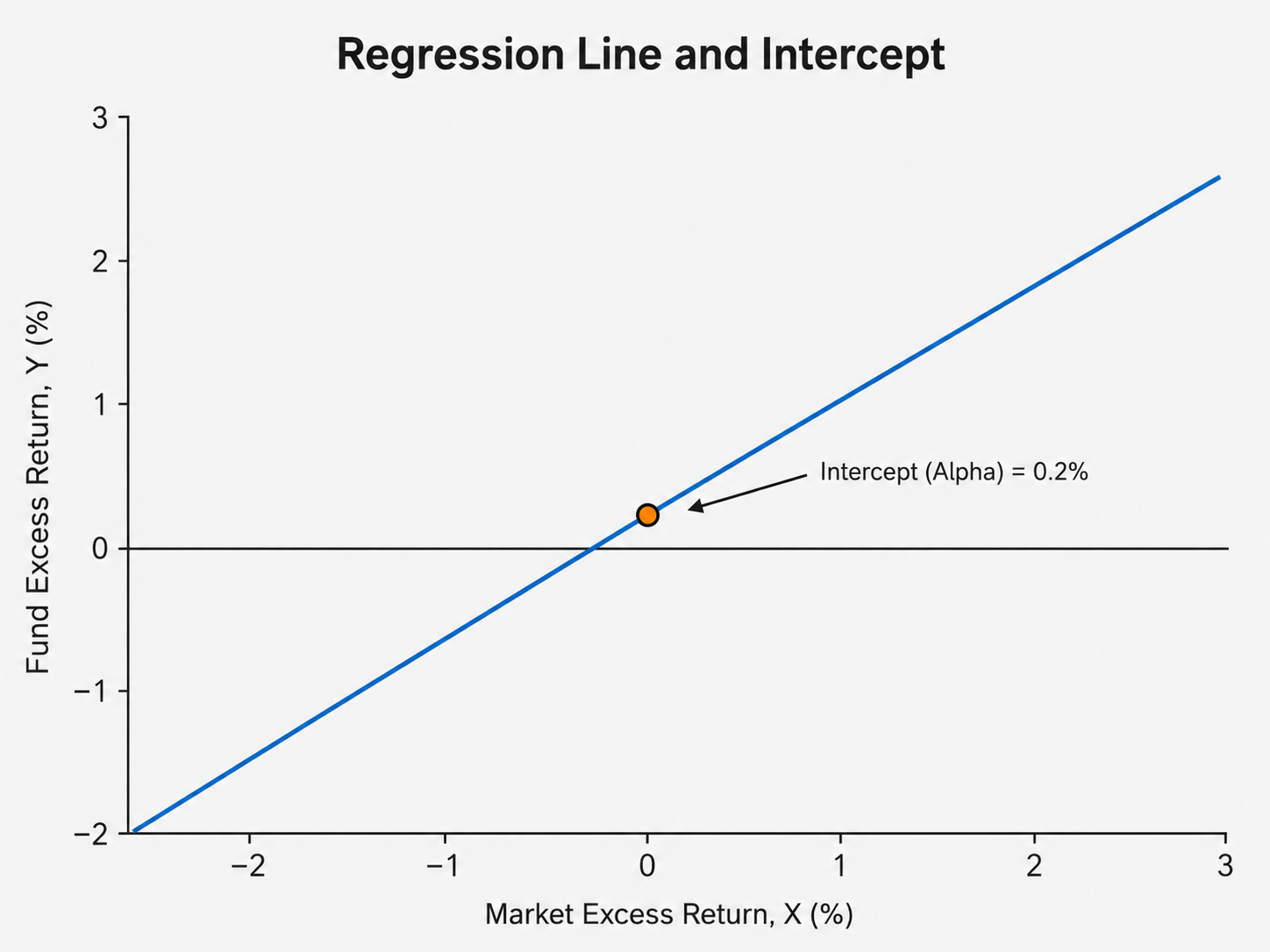
The regression line does not have to pass through the origin, which is the point (0, 0). In this example, the line crosses the Y-axis slightly above the origin because the estimated intercept is positive.
Alpha Is the Regression Intercept
In an investment regression, the intercept is normally called alpha.
Alpha = Regression intercept
They are not two separate calculations.
In the example:
Alpha = 0.2%
This means that when the market’s excess return is zero, the regression predicts that the fund’s excess return will be 0.20%.
A more useful investment interpretation is:
‘Alpha is the estimated average return that is not explained by the factors included in the regression.’
The final part of that definition is important. Alpha is the return unexplained by the particular model being used.
It is not necessarily a return that cannot be explained by any model.
A positive alpha does not automatically prove that an active manager has skill. It simply means that some average return remains unexplained after accounting for the variables included in the regression.
That unexplained return could arise because of:
genuine investment skill;
random luck;
a short or favourable sample period;
exposure to a factor omitted from the model;
an unsuitable benchmark;
stale pricing;
data errors;
selection bias;
or data-mining.
It is therefore safer to describe alpha initially as ‘unexplained return’, rather than immediately calling it manager skill.
Beta: The Slope of the Regression Line
Beta is the slope of the regression line.
It measures how much Y tends to change when X changes by one unit.
Using the example:
Y = 0.2% + 0.86X
the beta is:
Beta = 0.86
This means that a 1 percentage point increase in the market’s excess return is associated with an estimated 0.86 percentage point increase in the fund’s excess return.
Suppose the market excess return is 2%.
Y = 0.2% + 0.86(2%)
Y = 0.2% + 1.72%
Y = 1.92%
The regression therefore predicts a fund excess return of 1.92%.
The use of phrasing here is very important, as outlined below.
A return of 1.00% rising to 2.00% represents an increase of 1 percentage point. It does not represent an increase of 1%.
In relative terms, however, the return has increased by 100%:
(2.00% - 1.00%) / 1.00% = 100%
It has doubled from 1.00% to 2.00%. It has not increased by 1%.
A market beta can be interpreted approximately as follows:
Beta = 1.00 — The investment tends to move approximately one-for-one with the market.
Beta = 0.80 — The investment tends to move 20% less than the market.
Beta = 1.20 — The investment tends to move 20% more than the market.
Beta = 0.00 — There is no estimated linear relationship with the market.
Beta below 0 — The investment tends to move in the opposite direction to the market.
A beta of 0.86 does not mean that the fund will always rise by exactly 0.86% whenever the market rises by 1%. It describes the estimated average relationship across the full sample.
Predicted Values
The regression equation can be used to calculate a predicted value of Y.
The predicted value is often written as Ŷ.
Predicted Y = α̂ + β̂X
The word ‘hat’ indicates that alpha and beta have been estimated from a sample. They are not values known with certainty.
Using the example:
Predicted Y = 0.2% + 0.86X
Suppose the market excess return is 1%.
Predicted Y = 0.2% + 0.86(1%)
Predicted Y = 1.06%
The regression predicts that the fund will earn an excess return of 1.06%.
The fund’s actual return may be higher or lower.
The Error Term and Residual
Real investment returns rarely sit exactly on a regression line.
The complete simple regression is:
Y = alpha + beta X + error
The error term represents the part of Y that the model does not explain.
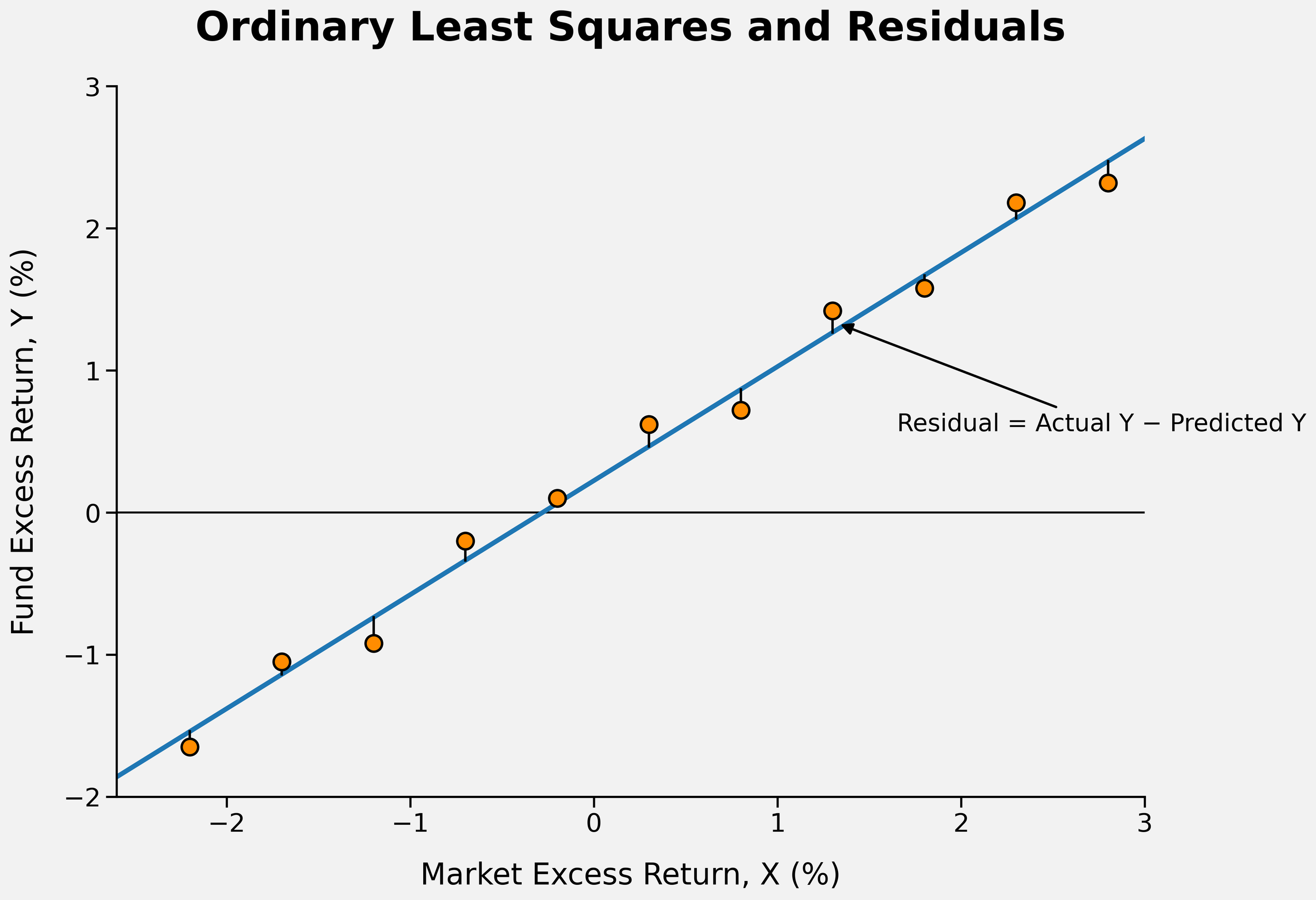
Once the regression has been estimated, the difference between the actual value and the predicted value is called the residual.
Residual = Actual Y - Predicted Y
Suppose:
Market excess return = 1.00%
Predicted fund excess return = 1.06%
Actual fund excess return = 1.35%
The residual is:
Residual = 1.35% - 1.06%
Residual = 0.29%
The actual fund return was 0.29 percentage points higher than the model predicted.
A positive residual means that the fund performed better than the model predicted during that particular period.
A negative residual means that the fund performed worse than the model predicted.
This gives us the relationship:
Actual return = Predicted return + Residual
In this example:
1.35% = 1.06% + 0.29%
A residual for one month is not the same as alpha.
Alpha is the estimated average intercept across the full sample.
Residuals are the individual period-by-period prediction errors.
A fund can have an alpha close to zero whilst still experiencing large positive and negative residuals from month to month. The residuals may largely cancel out over time, leaving little or no consistent unexplained return.
Strictly speaking, an error term is the unknown difference between an observation and the value predicted by the true relationship across all possible observations (the population model). A residual is the difference we can calculate using the estimated regression fitted to the sample of data available to us.
In practical fund analysis, however, the two terms are often used interchangeably.
How Does the Regression Choose the Line?
There are many possible straight lines that could be drawn through a group of observations.
The regression therefore needs a rule for choosing the best one.
The most common method is ordinary least squares, usually shortened to OLS.
For every observation, the regression calculates the difference between the actual Y-value and the predicted Y-value.
Residualₜ = Actual Yₜ − Predicted Yₜ
It then squares each residual.
Squared residualₜ = (Actual Yₜ − Predicted Yₜ)²
Finally, it adds all the squared residuals together.
Sum of squared residuals = Σ (Actual Yₜ − Predicted Yₜ)²
OLS chooses the alpha and beta values that make this total as small as possible.
In simple terms, it finds the line that minimises the total squared vertical distance between the observations and the regression line.
The word ‘vertical’ matters because the regression measures the distance between each actual Y-value and the value of Y predicted by the line at that particular X-value.
Why Are the Residuals Squared?
Squaring the residuals does two useful things.
First, it prevents positive and negative errors from cancelling one another out.
Without squaring:
+2 + (-2) = 0
This would misleadingly suggest that there was no error.
After squaring:
2² + (−2)² = 4 + 4 = 8
Second, squaring gives greater weight to large errors.
1² = 1
4² = 16
An error of four is therefore treated as much more serious than an error of one.
OLS does not simply draw a line that looks sensible. It applies a mathematical rule to estimate the intercept and slope that produce the smallest possible sum of squared residuals.
Correlation Versus Regression
Correlation and regression are related, but they are not the same.
Correlation measures how closely two variables move together.
It normally ranges from -1 to +1.
Correlation = +1 A perfect positive linear relationship.
Correlation = 0 No linear relationship.
Correlation = -1 A perfect negative linear relationship.
Correlation treats the two variables symmetrically.
It does not formally describe one variable as the thing being explained and the other as the explanatory variable.
Regression assigns different roles.
Y = The variable being explained
X = The explanatory variable
Regression also produces an estimated equation.
Predicted Y = 0.2% + 0.86X
Correlation tells us how strongly two variables move together.
Regression tells us the estimated slope, intercept and predicted value of Y.
Neither correlation nor regression proves causation. A statistical relationship can appear because one variable influences another, but it can also appear because both variables are influenced by something else or because the relationship occurred by chance.
Multiple Regression
A simple regression has one X-variable.
Y = α + β₁X₁ + ε (error term)
A multiple regression contains more than one X-variable.
Y = α + β₁X₁ + β₂X₂ + β₃X₃ + ε
The principle remains the same.
Y is still the variable being explained.
The difference is that the regression now uses several explanatory variables simultaneously.
This is what happens in a Fama–French factor regression.
The Fama–French Three-Factor Regression
The Fama–French three-factor regression can be written as:
Rᵢ,ₜ − Rᶠ,ₜ = αᵢ + βMKT(Rₘ,ₜ − Rᶠ,ₜ) + βSMB·SMBₜ + βHML·HMLₜ + εᵢ,ₜ
Although the equation looks more complicated, its basic structure is still:
Y = α + β₁X₁ + β₂X₂ + β₃X₃ + ε
The left-hand side contains the return being explained. The right-hand side contains the intercept, the factor returns and their estimated coefficients.
Y: The Investment’s Excess Return
The dependent variable is:
Rᵢ,ₜ − Rᶠ,ₜ
This is the fund, stock or portfolio return above the risk-free return.
Investment excess return = Investment return − Risk-free return
For each month, the investment’s excess return becomes one Y-observation.
X₁: The Market Excess Return
The first explanatory variable in the Fama-French Three Factor Model is:
Rₘ,ₜ − Rᶠ,ₜ
This is the broad equity market’s return above the risk-free return.
Market excess return = Market return − Risk-free return
The coefficient attached to this factor is the market beta.
βMKT = the investment’s estimated sensitivity to the market excess return
X₂: SMB
The second explanatory variable is:
SMBₜ
SMB means ‘small minus big’.
It represents the return difference between diversified portfolios of smaller companies and larger companies.
A positive SMB return means that smaller companies outperformed larger companies during that period.
A negative SMB return means that larger companies outperformed smaller companies.
The coefficient attached to SMB measures how strongly the investment behaves like the small-company factor.
Positive βSMB = the investment behaves more like smaller companies
Negative βSMB = the investment behaves more like larger companies
X₃: HML
The third explanatory variable is:
HMLₜ
HML means ‘high minus low’.
It represents the return difference between high book-to-market value companies and low book-to-market growth companies.
A positive HML return means that value companies outperformed growth companies during that period.
A negative HML return means that growth companies outperformed value companies.
The coefficient attached to HML measures the investment’s estimated value exposure.
Positive βHML = the investment behaves more like value companies
Negative βHML = the investment behaves more like growth companies
These factors are not simply invented statistical series. Fama and French construct them from diversified portfolios of stocks sorted by size and book-to-market characteristics (Fama and French 1993). Please see my other post entitled ‘How Fama and French Build Portfolios’.
Interpreting a Fama–French Regression
Suppose a regression produces the following equation:
Fund excess return = 0.10% + 0.95(Market excess return) + 0.30(SMB) + 0.45(HML) + residual
Each coefficient has a separate interpretation.
Alpha: 0.10%
The regression estimates an unexplained excess return of 0.10% per month.
This is the intercept.
The model predicts an excess return of 0.10% when the market, SMB and HML factor returns are all zero.
It does not mean that the fund earns exactly 0.10% of alpha every month. It is an estimated average across the full sample.
Market Loading: 0.95
The fund has slightly less market sensitivity than a portfolio with a market beta of 1.00.
A 1 percentage point increase in the market excess return is associated with an estimated 0.95 percentage point increase in the fund’s excess return, holding the other factor returns constant.
SMB Loading: 0.30
The fund has positive exposure to the size factor.
Its returns behave partly like a portfolio tilted towards smaller companies.
The coefficient does not mean that 30% of the fund is invested in small companies. It measures sensitivity to the returns of the SMB factor, not a literal portfolio weight.
HML Loading: 0.45
The fund has positive exposure to the value factor.
Its returns behave partly like a portfolio tilted towards value companies.
Again, this is a return sensitivity rather than a direct statement that 45% of the portfolio is invested in value stocks.
A Complete Monthly Calculation
Assume that the estimated regression is:
Fund excess return = 0.10% + 0.95(Market excess return) + 0.30(SMB) + 0.45(HML)
Now suppose the factor returns during a particular month are:
Market excess return = 2.00%
SMB return = 1.00%
HML return = −0.50%
The model’s predicted fund excess return is:
Predicted fund excess return = 0.10% + 0.95(2.00%) + 0.30(1.00%) + 0.45(−0.50%)
Calculate each component separately.
Market contribution = 0.95 × 2.00% = 1.90%
SMB contribution = 0.30 × 1.00% = 0.30%
HML contribution = 0.45 × −0.50% = −0.225%
Now add the components together.
Predicted fund excess return = 0.10% + 1.90% + 0.30% − 0.225%
Predicted fund excess return = 2.075%
The model predicts an excess return of approximately 2.08%.
Suppose the fund actually earns an excess return of 2.30%.
Residual = Actual return − Predicted return
Residual = 2.30% − 2.075%
Residual = 0.225%
The fund performed 0.225 percentage points better than the model predicted during that month.
That one positive residual is not alpha. Alpha is estimated from the relationship across all the observations in the sample.
What Does ‘Holding Everything Else Constant’ Mean?
Multiple regression estimates each coefficient whilst accounting for the other variables included in the model.
Suppose the SMB coefficient is 0.30.
The proper interpretation is:
‘A 1 percentage point increase in SMB is associated with a 0.30 percentage point increase in the fund’s excess return, holding the market and HML factor returns constant.’
This qualification matters because investment factors can move together.
Smaller companies may sometimes perform well during the same periods as value companies. A fund’s returns might therefore be correlated with both SMB and HML.
Multiple regression attempts to separate these overlapping relationships. The SMB coefficient measures the fund’s estimated relationship with SMB after accounting for its relationships with the market and HML.
The coefficients are estimated together.
The regression is not normally run once using the market, once using SMB and once using HML, with the results simply added together. That would fail to account properly for the relationships between the explanatory variables.
Instead, all three factors are included in the same multiple regression. This allows the model to estimate the fund’s sensitivity to each factor whilst controlling for its exposure to the others.
What Does R² Mean?
R², pronounced ‘R-squared’, measures how much of the variation in Y is explained by the regression.
It is usually expressed between zero and one, or between 0% and 100%.
Suppose a regression produces:
R² = 0.90
This means:
‘Approximately 90% of the variation in the fund’s returns during the sample is explained by the factors included in the model.’
The remaining variation is not explained by those factors.
An R² of 0.30 means that the model explains much less of the fund’s historical return variation.
It is important to be precise about what R² does not mean.
An R² of 90% does not mean:
90% of the fund’s total return came from the factors;
the model is 90% accurate;
future returns are 90% predictable; or
there is a 90% probability that the model is correct.
R² concerns the historical variation in returns, not the amount of return earned.
A broad passive equity fund would usually be expected to have a high R² relative to an appropriate equity factor model. A concentrated, market-neutral or unusual strategy may have a lower R² because a greater proportion of its return variation is not captured by the factors.
A high R² is not automatically good and a low R² is not automatically bad. It depends on what the strategy is trying to achieve and whether the factors are appropriate.
Standard Errors
Regression coefficients are estimates calculated from a sample.
If the regression were run using a different period, the estimated alpha and factor loadings would probably change.
The standard error measures the uncertainty around a coefficient estimate.
Suppose the estimated monthly alpha is:
Alpha = 0.10%
with a standard error of:
Standard error = 0.08%
The alpha estimate is small relative to its uncertainty.
Now suppose the same alpha has a standard error of only 0.02%.
Alpha = 0.10%
Standard error = 0.02%
The estimate is much larger relative to its uncertainty.
Smaller standard errors indicate more precise estimates.
Standard errors are affected by several things, including:
the number of observations;
the level of unexplained noise;
how much the factor returns vary;
the correlation between explanatory variables; and
whether the assumptions used to calculate the standard errors are appropriate.
Financial return data can contain changing volatility and correlation through time. For that reason, academic and professional analyses may use adjusted standard errors, such as heteroskedasticity-consistent or Newey–West standard errors, rather than relying only on the simplest OLS calculation.
The t-Statistic
The t-statistic compares a coefficient estimate with its standard error.
t-statistic = Estimated coefficient ÷ Standard error
Suppose monthly alpha is:
Alpha = 0.10%
and its standard error is:
Standard error = 0.05%
Then:
t-statistic = 0.10 ÷ 0.05
t-statistic = 2.0
A larger absolute t-statistic means that the coefficient is large relative to its estimated uncertainty.
As a rough traditional rule, an absolute t-statistic near or above two is often treated as evidence that a coefficient is statistically different from zero at approximately the 5% level. The precise threshold depends on the sample size and statistical assumptions.
The absolute value matters because a strongly negative coefficient can also be statistically significant.
For example:
t = 0.4 — Weak evidence that the coefficient differs from zero.
t = 1.2 — Generally weak evidence.
t = 2.1 — Conventionally described as statistically significant.
t = −3.0 — Strong evidence of a negative coefficient.
Statistical significance does not automatically mean economic significance.
A very small coefficient can be statistically significant if it is estimated very precisely.
A large coefficient can be statistically insignificant if the data are noisy.
The p-Value
The p-value is closely related to the t-statistic.
The calculation begins with a null hypothesis. For a regression coefficient, the null hypothesis is usually:
Null hypothesis: the true coefficient is zero.
In other words, the null hypothesis assumes that there is no genuine relationship between that explanatory variable and the fund’s return, after accounting for the other variables in the model.
The p-value then asks:
‘If the null hypothesis were true, how unusual would it be to observe a coefficient estimate at least as far from zero as the one found in the sample?’
A small p-value means that the observed estimate would be relatively unusual if the true coefficient were zero. This provides evidence against the null hypothesis.
A conventional threshold is:
p-value < 0.05
When the p-value is below 0.05, the result is commonly described as statistically significant and the null hypothesis is rejected at the 5% significance level. This threshold is a convention, however, rather than a law of nature.
A p-value does not tell us:
the probability that the null hypothesis is true;
the probability that the coefficient is true;
the probability that the result occurred by chance;
the probability that a manager has skill; or
whether the result will continue in the future.
Instead, it tells us how compatible the observed data are with the null hypothesis that the true coefficient is zero.
Confidence Intervals
A confidence interval provides a range of values that are reasonably consistent with the estimated coefficient and the uncertainty surrounding it.
A rough 95% confidence interval can be calculated as:
Estimated coefficient ± 2 × Standard error
Suppose alpha is:
Alpha = 0.10%
and its standard error is:
Standard error = 0.08%
The approximate interval is:
0.10% ± 2(0.08%)
0.10% ± 0.16%
This gives an approximate range of:
−0.06% to 0.26%
The range includes zero. In this context, an alpha of zero means that the fund has no estimated abnormal return after accounting for its factor exposures.
Because zero is one of the values that remains reasonably consistent with the data, there is not enough evidence to conclude that the fund’s true alpha is different from zero at the 5% significance level.
This does not prove that the true alpha is zero. It means that the estimate is too uncertain to distinguish reliably between a negative alpha, no alpha and a positive alpha.
Now suppose the estimated alpha is:
Alpha = 0.20%
and its standard error is:
Standard error = 0.05%
The approximate 95% confidence interval is:
0.20% ± 2(0.05%)
0.20% ± 0.10%
This gives an approximate range of:
0.10% to 0.30%
This range does not include zero. Every value within the interval is positive, so the data provide stronger evidence that the fund’s true alpha is greater than zero. The result would therefore normally be described as statistically significant at approximately the 5% level.
The interval still does not prove that the true alpha lies within this particular range, nor does it prove that the manager has skill or that the positive alpha will continue. It shows that a true alpha of zero is not reasonably consistent with the estimate under the assumptions of the regression model.
These examples also show why focusing only on the point estimate can be misleading. Two funds may both have positive estimated alphas, but the estimate with the narrower confidence interval provides more precise evidence about the likely size and direction of the true coefficient.
Why Excess Returns Are Used
Factor regressions normally use returns above the risk-free rate because the model is trying to explain compensation for bearing risk.
Suppose:
Fund return = 1.00%
Risk-free return = 0.20%
Then:
Fund excess return = 1.00% − 0.20% = 0.80%
The regression is trying to explain the 0.80% earned above the risk-free return.
The market factor is also normally measured as an excess return.
Market excess return = Market return − Risk-free return
SMB and HML are already long-short return spreads. They represent the difference between two groups of stocks, so the risk-free rate is not separately subtracted from them.
Why Alpha Changes When Factors Are Added
Suppose a CAPM regression contains only the market factor.
Fund excess return = α + βMKT(Market excess return) + ε
The model accounts for market exposure, but not for size, value or other systematic return patterns.
Now add SMB and HML.
Fund excess return = α + βMKT(Market excess return) + βSMB(SMB) + βHML(HML) + ε
The estimated alpha may fall.
For example:
CAPM alpha = 0.30% per month
Fama–French three-factor alpha = 0.12% per month
Five-factor alpha = 0.04% per month
This does not necessarily mean that the original CAPM regression was calculated incorrectly.
It means that the simpler model attributed more of the fund’s return to the intercept because it contained fewer explanatory variables.
Once size and value exposures are included, some of the return previously labelled alpha may be explained as compensation associated with systematic factor exposure.
Alpha is therefore model-dependent.
A fund can have positive alpha under one model and little or no alpha under another.
This is one reason why claims of manager skill need to be treated carefully. The conclusion may depend on which factors are included in the regression and whether those factors capture the strategy’s true exposures.
Regression Does Not Prove Causation
A regression identifies statistical relationships.
It does not automatically prove that X causes Y.
A fund may have a strong positive HML loading because it deliberately invests in value stocks. In that case, there is a sensible economic explanation for the statistical relationship.
However, regressions can also identify relationships that arise because of:
coincidence;
omitted variables;
shared exposure to another source of risk;
data-mining;
reverse causality;
unusual sample periods; or
unsuitable data.
Regression results should therefore be interpreted alongside investment theory, portfolio holdings and economic reasoning.
A coefficient that has no credible economic explanation should not be accepted simply because it has a large t-statistic.
What a Factor Regression Is Really Doing
A factor regression divides an investment’s return into three broad parts.
Investment return = Alpha + Factor-related return + Residual
More precisely:
Alpha = the estimated average intercept
Factor loadings = the investment’s estimated systematic exposures
Residual = the period-by-period difference between actual and predicted returns
The regression is effectively asking:
‘What combination of factor exposures best recreates the pattern of returns we observed, and is anything consistently left over?’
That final part is where alpha enters.
If the factor model explains the return pattern well, the intercept should be close to zero and the residuals should fluctuate around zero without leaving a persistent pattern.
If the intercept is positive and statistically reliable, the model has not fully explained the average return. That may be evidence of skill, but it may also mean that the model is incomplete.
The Most Important Terms
The core ideas can be summarised as follows.
Y = the variable being explained
X = a variable used to explain Y
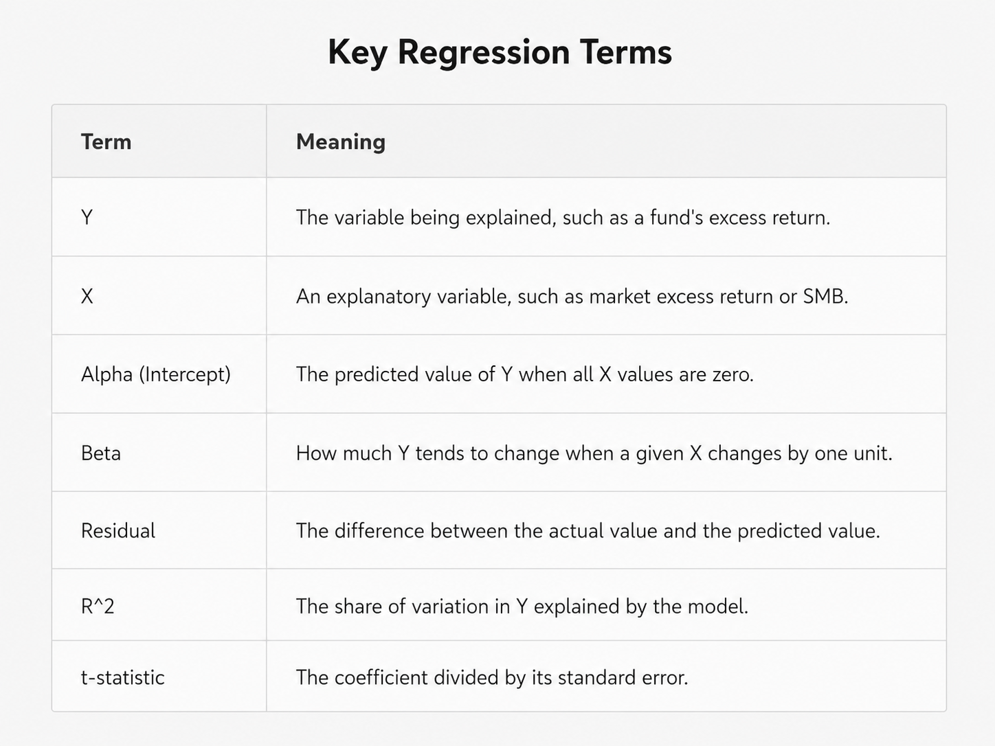
Intercept = the predicted value of Y when all X-values equal zero
Alpha = the intercept in an investment factor regression
Beta or coefficient = the estimated sensitivity of Y to an X-variable
Predicted value = the value produced by the regression equation
Residual = actual value minus predicted value
OLS = the method that chooses coefficients by minimising squared residuals
R² = the share of variation in Y explained by the model
Standard error = the estimated uncertainty around a coefficient
t-statistic = the coefficient divided by its standard error
p-value = evidence about how unusual the result would be if the true coefficient were zero
Confidence interval = a range of plausible values around the estimate
Multiple regression = a regression containing more than one explanatory variable
Conclusion
Regression equations can look technical, but the underlying structure is relatively straightforward.
Y is the return we want to explain.
X represents the variable, or variables, used to help explain it.
Beta measures how sensitive Y is to each X-variable.
Alpha is the intercept, which represents the estimated average return left unexplained by the factors included in the model.
Residuals are the individual period-by-period differences between actual and predicted returns.
R² tells us how much of the historical variation in returns is explained by the model, whilst standard errors and t-statistics help us judge how uncertain the estimated coefficients are.
A Fama–French regression is therefore not fundamentally different from a simple straight-line regression. It simply contains several X-variables rather than one.
The basic question remains the same:
‘What combination of exposures best explains the return pattern we observed, and is anything consistently left over?’
Understanding that question makes the equations much easier to interpret. It also helps prevent alpha, statistical significance and R² from being given more meaning than they deserve.
References
Fama, Eugene F., and Kenneth R. French. 1992. ‘The Cross-Section of Expected Stock Returns’. The Journal of Finance 47 (2): 427–465.
Fama, Eugene F., and Kenneth R. French. 1993. ‘Common Risk Factors in the Returns on Stocks and Bonds’. Journal of Financial Economics 33 (1): 3–56.
Fama, Eugene F., and Kenneth R. French. 2015. ‘A Five-Factor Asset Pricing Model’. Journal of Financial Economics 116 (1): 1–22.
Sharpe, William F. 1964. ‘Capital Asset Prices: A Theory of Market Equilibrium under Conditions of Risk’. The Journal of Finance 19 (3): 425–442.
Appendix
The estimated regression line does not include the residual:
Predicted Yₜ = α + βXₜ
For these five observations, the estimated regression line is:
Predicted Yₜ = 0.20% + 0.86Xₜ
Step 1: Calculate the Average Market Excess Return
Average X = Sum of X values / Number of observations
Average X = (-2.0% + -1.0% + 0.0% + 1.0% + 2.0%) / 5
Average X = 0.0% / 5
Average X = 0.0%
Step 2: Calculate the Average Fund Excess Return
Average Y = Sum of Y values / Number of observations
Average Y = (-1.5% + -0.7% + 0.2% + 1.1% + 1.9%) / 5
Average Y = 1.0% / 5
Average Y = 0.20%
Step 3: Calculate Beta
Beta measures how much the fund excess return tends to change when the market excess return changes.
The formula is:
β = Sum[(Xₜ - Average X)(Yₜ - Average Y)] / Sum[(Xₜ - Average X)²]
Because Average X = 0.0%, the calculations are simpler.
For Month 1:
X₁ - Average X = -2.0% - 0.0% = -2.0%
Y₁ - Average Y = -1.5% - 0.2% = -1.7%
(-2.0 × -1.7) = 3.4
(-2.0)² = 4.0
For Month 2:
X₂ - Average X = -1.0% - 0.0% = -1.0%
Y₂ - Average Y = -0.7% - 0.2% = -0.9%
(-1.0 × -0.9) = 0.9
(-1.0)² = 1.0
For Month 3:
X₃ - Average X = 0.0% - 0.0% = 0.0%
Y₃ - Average Y = 0.2% - 0.2% = 0.0%
(0.0 × 0.0) = 0.0
(0.0)² = 0.0
For Month 4:
X₄ - Average X = 1.0% - 0.0% = 1.0%
Y₄ - Average Y = 1.1% - 0.2% = 0.9%
(1.0 × 0.9) = 0.9
(1.0)² = 1.0
For Month 5:
X₅ - Average X = 2.0% - 0.0% = 2.0%
Y₅ - Average Y = 1.9% - 0.2% = 1.7%
(2.0 × 1.7) = 3.4
(2.0)² = 4.0
Now add the cross-products together:
Sum[(Xₜ - Average X)(Yₜ - Average Y)]
= 3.4 + 0.9 + 0.0 + 0.9 + 3.4
= 8.6
Now add the squared differences in X together:
Sum[(Xₜ - Average X)²]
= 4.0 + 1.0 + 0.0 + 1.0 + 4.0
= 10.0
Therefore:
β = 8.6 / 10.0
β = 0.86
Step 4: Calculate Alpha
The formula for alpha is:
α = Average Y - β(Average X)
Substitute the values:
α = 0.20% - 0.86(0.0%)
α = 0.20%
The intercept is therefore 0.20%.
This means that when the market excess return is 0%, the regression predicts that the fund excess return will be 0.20%.
Step 5: Write the Regression Line
The estimated regression line is:
Predicted Yₜ = α + βXₜ
Predicted Yₜ = 0.20% + 0.86Xₜ
The beta of 0.86 means that a one-percentage-point increase in the market excess return is associated with an estimated 0.86-percentage-point increase in the fund excess return.
The alpha of 0.20% means that the fund is predicted to produce an excess return of 0.20% when the market excess return is 0%.
For example, when the market excess return is 2.0%:
Predicted Yₜ = 0.20% + 0.86(2.0%)
Predicted Yₜ = 0.20% + 1.72%
Predicted Yₜ = 1.92%
The fund’s actual excess return in that month is 1.90%, which is very close to the value predicted by the regression line.
Another Scenario for Completeness
One slightly confusing point is what it means to ‘set X equal to zero’.
This does not mean changing the original observations. The five monthly returns remain exactly as they are. Instead, once the regression line has been estimated, we can use that fitted line to ask a simple question:
What fund excess return would the regression predict if the market excess return were 0%?
The fitted regression line is:
Predicted Y = α + βX
If X is set to zero, the equation becomes:
Predicted Y = α + β(0)
Predicted Y = α
So the predicted value of Y when X is 0% is simply the intercept, or alpha.
This is why alpha is often described as the estimated return when the market excess return is zero. In the example above, the fitted regression line is:
Predicted Y = 0.20% + 0.86X
If the market excess return is 0%, then:
Predicted Y = 0.20% + 0.86(0%)
Predicted Y = 0.20%
The regression therefore estimates that, when the market excess return is 0%, the fund excess return is 0.20%.
The same logic applies when the average market return is not zero. Regression estimates the line so that it passes through the average point:
(Average X, Average Y)
This means:
Average Y = α + β(Average X)
Rearranging gives:
α = Average Y − β(Average X)
For example, suppose the average market excess return was 0.50%, the average fund excess return was 0.80%, and beta was 0.90.
Then:
α = 0.80% − 0.90(0.50%)
α = 0.80% − 0.45%
α = 0.35%
The fitted line would therefore be:
Predicted Y = 0.35% + 0.90X
Setting X equal to zero gives:
Predicted Y = 0.35% + 0.90(0%)
Predicted Y = 0.35%
So ‘setting X equal to zero’ simply means using the estimated regression line to calculate the predicted value of Y when the market excess return is zero. It does not mean altering the original data.