Factor investing is built on the observation that certain groups of stocks systematically earn higher returns than others. The Capital Asset Pricing Model (CAPM) assumes that a single factor—the market portfolio—explains the cross-section of returns. Yet decades of evidence show that the CAPM leaves a large amount of the cross-section unexplained. For example, the fact that smaller companies tend to outperform larger companies as well as the observation that value stocks (measured by price-to-book) tend to outperform growth stocks. Fama and French (1993) formalised this in their three-factor model which takes into account the market, size and value factors to explain the cross-section of returns.

Even so, other anomalies remained. The three-factor model fails to explain portfolios sorted on profitability or investment intensity. Fama and French (2015) therefore extended their framework into a five-factor model by adding two ‘quality’ dimensions: profitability (RMW—robust minus weak) and investment (CMA—conservative minus aggressive). This model explains the cross-section more effectively than its predecessors. Crucially, it reduces the stand-alone importance of the traditional value factor, showing that much of what value captures is better explained by profitability and investment.

For investors, the key questions may be: What do these premia represent? How large are they? And can they be cost-efficiently captured and delivered as an investable product?

What Are Factor Premia?

A factor premium is the excess return earned by systematically tilting towards one characteristic of firms and away from its opposite. In academic tests, it is defined as the average return of a long–short portfolio—long the top 30% of firms by a characteristic, short the bottom 30%. For example, the profitability premium is the return of highly profitable firms minus the return of weakly profitable firms, controlling for market, size and value.

Measured in this way, premia are not abstract artefacts: they represent persistent differences in realised returns over decades. In practice, investors cannot directly run long–short portfolios, but they can capture the premium by overweighting the ‘long’ side and underweighting or excluding the ‘short’ side in long-only funds.

The Profitability Premium (RMW)

Construction. Profitability is measured as operating profits relative to book equity. The RMW factor goes long the most profitable firms (top 30%) and short the least profitable (bottom 30%). Novy-Marx (2013) shows that gross profitability—revenues minus cost of goods sold, scaled by assets—is also a powerful measure.

Magnitude of the premium. Hou, Xue and Zhang (2015) find that RMW delivers around 0.25–0.30% per month—about 3–4% per year—in both US and international data. Studies covering 23 countries from 1987–2019 confirm that the premium is statistically significant in North America, Europe and Asia-Pacific. The effect applies across large and small companies, with Japan an exception where the evidence is weaker.

Economic rationale. Risk-based explanations suggest that robustly profitable firms face greater competitive threats and therefore require higher returns to entice would-be investors; a weak rationale in my opinion. A behavioural explanation is perhaps more compelling: investors underestimate the persistence of profitability, systematically over-estimate weak firms’ prospects and overpay for speculative ‘story stocks’.

Performance across regimes. Novy-Marx (2013) shows that US stocks with high gross profitability significantly outperform weakly profitable ones. Fama and French (2015) find that RMW is positive and significant from 1963 onwards. The factor also proves defensive—profitable firms declined less during the global financial crisis of 2008 and the COVID-19 crash of 2020. Unlike size or value, RMW demonstrates consistent positive returns across market regimes.

Relationship with other factors. RMW is uncorrelated with value, since many highly profitable firms are often growth stocks. Yet combining the two improves outcomes. Screening out cheap but unprofitable firms—so-called value traps—enhances value strategies. Albion Strategic Consulting (2022) note that integrating profitability alongside value increases expected returns and reduces tracking error.

*Figure 1.* Profitability vs Book-to-Market (Fama–French Factor Returns, 1963–2025). Both axes are in monthly percentage returns.
Each X on the chart represents one month of data between July 1963 and 2025.
**X-axis value (RMW)**: how much the high-profitability stocks outperformed (or underperformed) the low-profitability stocks in that month, measured as a monthly factor return in percent.
Example: if RMW = +0.8, then robustly profitable stocks beat weakly profitable stocks by 0.8% that month.
If RMW = –0.5, weakly profitable stocks actually outperformed by 0.5%.
**Y-axis value (HML):** how much the value stocks (high book-to-market) outperformed (or underperformed) the growth stocks (low book-to-market) in that same month.
Example: if HML = +1.2, value beat growth by 1.2% that month.
If HML = –0.7, growth outperformed by 0.7%.
So, taken together, the scatter shows how the monthly profitability premium and the monthly value premium moved together over more than 700 months. The lack of a clear slope (and a correlation coefficient of only ~0.17) is why we say profitability is essentially uncorrelated with value.
This tells us that **highly profitable firms are often priced like growth stocks (low B/M), so profitability doesn’t overlap with value.** That’s why in the Fama–French five-factor model, profitability adds explanatory power beyond value.

The Investment Premium (CMA)

Construction. The CMA factor is defined as conservative minus aggressive investment. Firms are ranked by annual asset growth, with the most conservative (lowest 30%) forming the long portfolio and the most aggressive (highest 30%) forming the short.

Magnitude of the premium. Fama and French (2015) show that CMA delivers around 0.2–0.3% per month—roughly 2–3.5% per year—in US data. Internationally, the premium is positive but less statistically robust than RMW. Hou, Xue and Zhang (2015) find that size matters: CMA is stronger in small caps (~0.37% per month) than in large caps (~0.11% per month).

Economic rationale. Under q-theory, firms with low discount rates invest more and earn lower returns, whilst firms with high discount rates invest less and earn higher returns. Intuitively, if a firm’s cost of capital is high, it will only undertake highly profitable projects; that’s the investment premium. Behavioural forces reinforce this: investors overpay for firms expanding aggressively and undervalue cautious firms with steady cash flows. Over-investment driven by overconfidence or empire-building can also lead to poor subsequent returns.

Performance across regimes. CMA is cyclical. It excels in risk-off environments that punish speculative growth, such as the dot-com bust of 2000–2002 and the 2022 rotation when higher interest rates hit cash-burning tech stocks. But it struggles in liquidity-fuelled bull markets—like the 2010s—when cheap debt financing supports aggressive expansion.

Overlap with value. CMA is highly correlated with the value factor. Conservative firms often look cheap, aggressive firms expensive. Fama and French (2015) show that CMA, together with RMW, absorbs much of the explanatory power previously attributed to value in the three-factor model.

Links to the Low-Volatility Anomaly

The profitability and investment factors also shed light on the so-called low-volatility anomaly. On the surface, low-beta or low-volatility strategies appear to deliver market-like returns with significantly less risk—a compelling proposition since, with lower volatility but the same return, compounding delivers higher long-term wealth.

Academic research shows, however, that the anomaly is not driven by volatility per se. Low-volatility stocks tend to be those of profitable firms that invest conservatively, whilst high-volatility stocks are often unprofitable and aggressively expanding. Hou, Xue and Zhang (2015) show that when RMW and CMA are controlled for, the alpha of low-volatility strategies largely disappears. In effect, the premium reflects quality, not volatility.

Practitioners reach the same conclusion. Gerard O’Reilly of Dimensional Fund Advisors notes that Dimensional took the low-volatility research ‘very seriously’, since the idea of achieving the same returns with less volatility—and thus higher compounded growth—is highly appealing. Yet their analysis (alongside Novy-Marx’s) finds that ‘the reasons that the low-volatility stocks historically came in with market-like returns was because of their value and profitability characteristics and not to do with the volatility characteristics themselves’ (Rational Reminder Podcast, episode 198, 2022).

O’Reilly highlights that low-volatility portfolios are not stable in their composition. Sometimes they look like value and high profitability—when they outperform strongly—and sometimes like growth and low profitability—when they underperform. Small growth firms in particular often screen as ‘low vol’ but deliver poor returns, dragging on the strategy. The implication is that investors should not assume low-volatility strategies will always provide market-like returns going forward.

The practical takeaway is that the anomaly is unreliable as a stand-alone strategy. Its historical returns are explained by underlying value and profitability exposures—which investors can capture more directly. As O’Reilly concludes, blending equities with fixed income may provide a more robust way of reducing volatility without sacrificing expected return.

Implementation for Investors

For UK investors, capturing these premia requires appropriate funds in order to do so:

Dimensional Fund Advisors now offers the Global High Profitability Lower Carbon ESG Screened Fund with a strong tilt to the profitability factor as evidenced below:
Quality ETFs such as the iShares MSCI World Quality Factor ETF (IWQU) emphasise high return on equity, stable earnings and low leverage—closely aligned with RMW and CMA. However, when running a Fama–French 5 factor regression on the fund, the results are somewhat questionable. In my opinion, this goes to show that definitions of ‘quality’ will vary and as such it is important for investors to ‘look under the hood’ to judge for themselves.
Value ETFs such as Vanguard’s Global Value Factor UCITS ETF (VVAL) capture much of the investment (CMA) factor indirectly through value exposure; that is, given the overlap between conservative investment and value.
Multi-factor ETFs combine value, quality and momentum, providing broad exposure in a single fund. Again, though, would-be investors would be wise to do their own due diligence.

The impact of costs should not be understated. Factor premia are only expected to be a couple of per cent per annum on average, so paying more than 0.5% in fees can erode a significant amount of their benefit. Turnover is another consideration: successful managers minimise costs through patient trading.

A common structure is to hold a global index core, with satellites in profitability/quality and value funds. For example, 70% global index, a 15% value tilt and a 15% quality tilt delivers diversified exposure to the major premia without excessive tracking error.

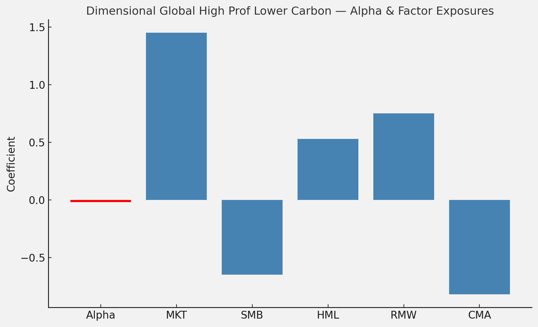
*Figure 2.* Dimensional Global High Profitability Lower Carbon ESG Screened Fund regression.
**What the regression is doing:**
I regressed the fund’s excess returns (fund return minus risk-free rate) on the Fama–French 5 factors (plus alpha):
Each coefficient (β) tells you how sensitive the fund is to that factor.
**Interpreting the coefficients we’ve got for this fund:**
*Alpha*: Slightly negative, close to zero. Suggests no evidence of excess return unexplained by the Fama–French 5 factors.
***MKT*** (~1.45): The fund loads more than one-for-one on the market factor. A coefficient > 1 just means it is more volatile / more sensitive to market moves than the market portfolio itself. This is quite normal for equity funds that take on systematic tilts (like profitability, smaller size, or non-US weightings). Think of it like a beta in the CAPM: >1 means higher market risk exposure.
***SMB***(~–0.6): Negative loading on size → fund tilts to large-cap stocks.
***HML*** (~0.5): Mild positive value tilt. Even though it’s branded ‘profitability,’ Dimensional often blends exposures to avoid uncompensated risks.
***RMW***(~0.75): Strong positive exposure to profitability—exactly what you’d expect.
***CMA*** (~–0.8): Negative investment loading, meaning preference for firms that invest more aggressively (not conservative investors). This is common for high profitability tilts.
***Why can the Market (MKT) coefficient be > 1?***
The regression coefficients are not constrained to 0–1; they reflect best fit to the historical data.
A β*MKT* > 1 means that the fund moves more than the market:
If the market goes up 1%, this fund tends to move ~1.45%.
If the market goes down 1%, same idea.
*Reasons for this*:
The fund has systematic tilts (profitability, some value) that increase volatility relative to the market in question.
The fund may also have a different regional mix than the market in question (e.g., more small/mid caps, more ex-US exposure).
Statistically, if the other factors don’t fully capture variation, the market factor absorbs it, pushing β above 1. See the appendix for further details on this phenomenon.

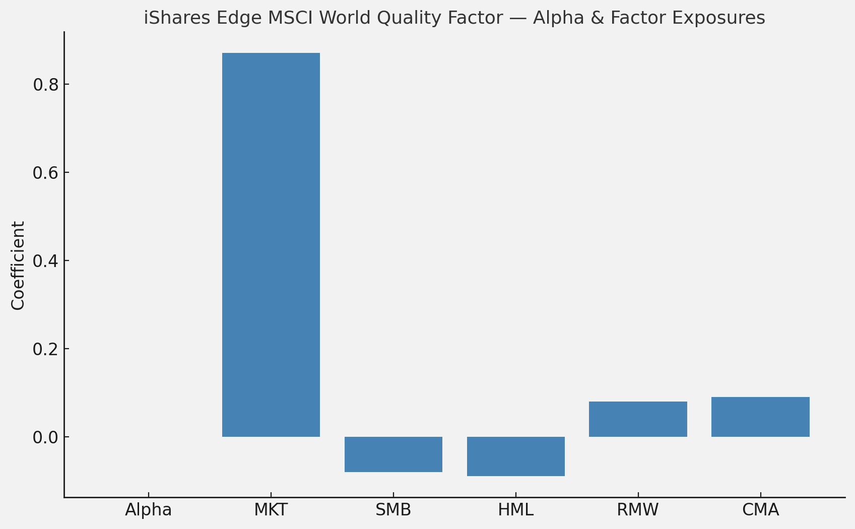
*Figure 3.* iShares Edge MSCI World Quality Factor regression.
The iShares ‘Quality’ fund does not load strongly on the Fama–French profitability (RMW) or investment (CMA) factors. This is because MSCI defines quality using a composite of return on equity, earnings stability and low leverage, which differs from the academic construction of profitability and investment premia. The result is a fund that looks much closer to the market, with only modest tilts, despite the ‘quality’ label.

*Figure 4.* Vanguard Global Value Factor regression.
The regression shows a clear value tilt (HML ≈ 0.4) alongside a size tilt (SMB ≈ 0.5), providing indirect exposure to the investment factor (CMA) given the overlap between conservative investment and value. However, there is only modest direct exposure to the profitability (RMW) and investment factors. Market exposure is below one, reflecting diversification but still broadly market-like behaviour. Alpha is negligible, suggesting returns are well explained by the Fama-French five-factor model.

Patience and Behaviour

The greatest challenge is behavioural. Both the profitability and investment factors can underperform for years. Investors who abandon these tilts during those periods risk missing the premium when it eventually reasserts itself. Vanguard (2021) caution that factor returns are cyclical and that harvesting them requires patience and discipline.

Conclusion

Profitability and investment premia reward investors for owning firms that generate sustainable earnings and avoiding those that pursue growth indiscriminately. They represent a significant advance on the CAPM and three-factor model, capturing dimensions of quality that other frameworks miss. Profitability has proven a consistent and defensive premium. Investment is more cyclical but valuable in avoiding overpriced growth traps. Together they explain much of the low-volatility effect and enhance portfolio efficiency.

As of September 2025—for UK investors, these premia are somewhat accessible through reasonably priced funds. Indeed, Dimensional’s Global High Profitability Lower Carbon ESG Screened fund seems to do a good job at capturing the profitability premium. Although, it should be stated that there doesn’t appear to be many good alternatives at present.

Interestingly, fund managers have largely steered clear of offering pure investment-factor funds. The practical difficulties of cleanly isolating asset growth, limited investor demand, overlapping signals with other factors and concerns about capacity likely explain why such funds are rare. For UK investors, the premium is somewhat accessible through reasonably priced multi-factor funds.

All in all, the evidence suggests that integrating profitability and investment can improve long-term outcomes—provided investors remain disciplined through inevitable economic cycles.

References

Albion Strategic Consulting. 2022. Governance Update #23.

Fama, Eugene, and Kenneth French. 1993. ‘Common Risk Factors in the Returns on Stocks and Bonds’. Journal of Financial Economics.

Fama, Eugene, and Kenneth French. 2006. ‘Profitability, Investment and Average Returns’. Journal of Financial Economics.

Fama, Eugene, and Kenneth French. 2015. ‘A Five-Factor Asset Pricing Model’. Journal of Financial Economics.

Hou, Kewei, Chen Xue, and Lu Zhang. 2015. ‘Digesting Anomalies: An Investment Approach’. Review of Financial Studies.

Novy-Marx, Robert. 2013. ‘The Other Side of Value: The Gross Profitability Premium’. Journal of Financial Economics.

Rational Reminder Podcast. 2022. ‘Dimensional Fund Advisors: Gerard O’Reilly’. Episode 198, 28 July. https://rationalreminder.ca/podcast/198

Vanguard. 2021. Factor-Based Investing: A Practitioner’s Guide.

Appendix: Why Missing Factors Distort Betas, Not Alpha

When interpreting factor regressions, it is important to understand what alpha and betas really represent.

Alpha (α) is the constant intercept in the regression. It can only capture a flat, average return unexplained by the included factors. Alpha does not move with market conditions.
Betas (β), by contrast, describe how the fund’s returns co-move with each factor over time. They rise and fall as the factors rise and fall.

This distinction matters because it explains why omitted factors do not appear in alpha. If a fund has exposure to a systematic source of returns that is not in the model (for example, momentum), that exposure is time-varying: it goes up and down with the omitted factor. A constant alpha cannot flex to fit this pattern.

Instead, the regression shifts the slope coefficients on the included factors, often inflating the market beta (βMKT) above one. In effect, the model makes the market factor ‘work harder’ to absorb variation that actually belongs to the missing factor.

Minimising error: Ordinary Least Squares (OLS) is designed to minimise squared errors. If stretching βMKT gives a closer fit than letting α absorb the variation, that is what the regression will do. Alpha can only capture a flat residual return, but the slope coefficients can bend to track time-varying co-movement.

The implication is clear. A high market beta may sometimes signal genuine greater sensitivity to equity risk, but it can also reflect exposures to systematic risks outside the model. This is why Eugene Fama and Kenneth French successively expanded their framework from three to five factors: the earlier models left structured variation that could only be properly explained by adding new dimensions.

Profitability and Investment Premia: What Fama–French’s ‘Quality’ Factors Mean for Investors